Outside Money, Inside Models

Why the DCF Systematically Misprices Gold Mining Companies

Abstract

The discounted cash flow model rests on the assumption that the cash flows in the numerator and the discount rate in the denominator share a common monetary reference frame. For most companies this assumption holds. For gold mining companies, it does not.

This paper argues that gold functions as outside money: its long-term price is determined by the confidence that external creditors place in the sustainability of the dollar-based monetary system rather than by industrial consumption or conventional inflation. Production costs, by contrast, remain fully anchored in the inside-money system. The standard WACC, built entirely from inside-money variables (Treasury yields, dollar equity risk premia, and equity betas), is therefore structurally mismatched to the revenue dynamics it is asked to discount.

The resulting error produces systematic undervaluation through two channels. The first is a misspecification of the gold price assumption, calibrated on a framework whose explanatory power has collapsed in institutional data since 2022. The second is a model specification error: the standard single-factor cost of capital, by structural design, omits the monetary regime factor to which gold mining revenues are negatively exposed. Both errors push valuation in the same direction. The distortion is largest precisely when gold’s protective characteristics are most valuable, and helps explain persistent P/NAV discounts even in the most stable mining jurisdictions and at record operating margins.

The paper distinguishes this architectural flaw from operational and jurisdictional risks, including the dollar-denominated debt of major producers, which constitutes a serious counterweight in specific monetary configurations. It addresses the principal objections, and reframes the in-situ valuation method not as a replacement for the DCF but as the empirical aggregate of DCFs run by acquirers operating outside the institutional constraints of sell-side research. It offers four testable predictions with explicit falsification conditions, including the specific monetary regime under which the standard model would recover its validity. A formal decomposition of the error is presented in Appendix A; three case studies (junior, mid-tier, senior) document the empirical signature.

The gap between what the standardized models say these companies are worth and what informed buyers pay for their ounces is not noise. It is the measure of the error.

Keywords: Discounted Cash Flow · Gold Mining Valuation · Monetary Regime Risk · Outside Money · WACC · Multi-Factor Asset Pricing · Fiscal Dominance · In-Situ Valuation · Petrodollar System

JEL classification: G12 (Asset Pricing) · G31 (Capital Budgeting) · G32 (Financing Policy) · Q31 (Mineral Resources) · E42 (Monetary Systems) · F33 (International Monetary Arrangements)

References follow Chicago author-date format. Online sources accessed May 2026.

Section I — The Instrument and Its Assumptions

How do you value a company?

The question sounds simple. It has been asked in every boardroom, every transaction process, every business school classroom since the concept of a going concern first acquired a market price. And beneath the complexity of every methodology ever devised (the comparable transactions, the trading multiples, the precedent deals), there is one answer that is both complete and irreducible.

A company is worth the cash it holds today plus the cash it will generate in the future, brought back to the value of today’s cash. Nothing more. Nothing less.

This is not a simplification. It is the definition. The discounted cash flow model is the attempt to make this definition operational, to convert a stream of future payments into a single present value through the application of a discount rate that reflects the time value of money and the risk of receiving those payments.

When the market prices a company above this value, it is paying for something that does not yet exist in the numbers: the possibility that operational leverage will compound, that management will find ways to generate cash beyond what current assets suggest. This excess is what accounting calls goodwill and what markets call expectation. It is the price of optionality. The first exercise of valuation is arithmetic, estimating what can be reasonably projected. The second is judgment, deciding what to pay for what cannot. The DCF handles the first. The market handles the second.

This paper is concerned with a structural flaw in the arithmetic itself. Not from optimistic assumptions or aggressive multiples, but because the model applies a single monetary reference frame to a cash flow stream whose two components, revenues and costs, do not, for one specific class of assets, inhabit the same monetary world.

To see the flaw, one must first understand the world for which the model was built.

Every economy is, at its foundation, energy transformed. Over five decades, global GDP has broadly tracked primary energy consumption and the stock of energy materialized in productive capital with striking regularity. Steel, semiconductors, pharmaceuticals, airline tickets, all are energy reorganized into value. The price of goods and services ultimately reflects the energy required to produce them.

Since 1974, that energy has been priced predominantly in one currency. The U.S.-Saudi agreement of that year, extended through the architecture of OPEC pricing conventions, contributed decisively to the dollarization of oil trade. Countries needing energy needed dollars. Exporters accumulated them, recycling them into Treasuries. The dollar became the currency of the closed energy loop: not by fiscal virtue, but because the physical economy runs on energy, and energy runs on dollars.

Within this closed loop, the DCF model is internally coherent. The weighted average cost of capital draws entirely from its components: the Treasury yield, dollar equity risk premia, betas against dollar indices. For major gold producers today, this produces a WACC between 7.5% and 9%. For the vast majority of companies, whose revenues and costs are both expressions of energy priced in the loop’s unit of account, the assumption holds. When the dollar loses purchasing power, both sides of the income statement adjust roughly in step. The model breathes with the system that surrounds it.

The embedded premise, that the dollar in the revenue line and the dollar in the discount rate are the same object, is so fundamental it is rarely stated. It does not need to be. It is true for most assets.

It fails for one specific class. Not marginally. Architecturally.

These assets incur costs fully anchored in the closed loop (wages, diesel, electricity, reagents, taxes) while their revenues derive from an output whose long-term price is driven not by the productivity of the loop but by the confidence external creditors place in its sustainability. This output rises when the loop’s external obligations outrun its capacity to honor them without devaluation.

The short-term volatility of this price is real. It is orthogonal to the argument. Over the fifteen-to-twenty-year horizon of a standard mining DCF, the divergence between the monetary world of costs and the monetary world of revenues is the signal, not the noise.

The discounted cash flow model, applied to the producers of this asset, therefore discounts revenues that respond to monetary regime risk at a rate constructed entirely within that regime. The numerator and the denominator do not share a common reference frame. This is not a problem of better inputs. It is a problem of architecture.

The asset, and the precise nature of this divergence, is the subject of what follows.

The tool still produces a number. The number is no longer the value.

Section II — Methodology and Scope

Before developing the substantive argument, the paper’s methodology and the choices that govern its evidentiary basis deserve explicit statement.

The argument advanced here is primarily analytical. Its contribution lies in identifying a structural mismatch in a widely used valuation model, not in producing new econometric estimates of the parameters that would calibrate the corrected model. Section IV develops a formal decomposition of the error in two channels (numerator and denominator), and Appendix A presents the corresponding equations in standard asset pricing notation. Empirical claims about the magnitude of the error are illustrated through three case studies (Section IV) covering different points of the producer spectrum, and triangulated against the convergent findings of four institutional sources.

The empirical evidence relies on a tiered hierarchy of sources, with explicit preference for institutional documentation that the reader can verify directly. Tier 1 sources (RBC Wealth Management, Apollo Academy, S&P Global Market Intelligence, and the World Gold Council) produce the four convergent findings on the post-2022 collapse of the gold-real yield framework that anchor Section IV. These sources were selected on three criteria: institutional independence (no shared data provider, no shared methodology), public verifiability (each finding can be located and cross-checked by any reader), and methodological diversity (each uses a different lens on the same phenomenon). Tier 2 sources (corporate filings such as PEA, 10-K, 6-K; exchange data; central bank disclosures) provide the quantitative inputs for the case studies. Tier 3 sources, in particular independent analysts such as Nieuwenhuijs on PBoC reserves and Momentum Structural Analysis on the GDX-to-gold spread, are explicitly flagged in footnotes and used only where Tier 1 and Tier 2 evidence is unavailable.

The period of empirical focus is 2022–2026, corresponding to the documented regime break in the gold-real yield relationship. Historical references (1971–1980, 2000–2011) appear in Section III to establish the structural mechanism, not to test the post-2022 hypothesis.

Three limitations of the present approach should be stated plainly. First, the paper does not produce a calibrated estimate of λ_monetary, the price of monetary regime risk, nor an empirical estimate of β_monetary for individual producers. It identifies the omission of these parameters as the structural defect in standard pricing, and proposes a multi-factor specification (Appendix A) that would accommodate them; their econometric estimation is left to subsequent work. Second, the empirical illustration relies on three case studies rather than a sectoral regression. The cases were chosen to span the producer spectrum (junior, mid-tier, senior) and to test the predicted relationship between balance-sheet exposure to dollar debt and the magnitude of mispricing; they are not a statistically representative sample. Third, the argument concerns long-cycle valuation under the regime documented from 2022 onward. It does not claim that the standard model has been wrong in all monetary regimes, Section VI specifies the regime under which the single-factor framework would recover its validity, and the empirical conditions that would invalidate the present thesis.

Section III — The Asset That Breaks the Assumption

Gold is not a commodity[1].

This statement will irritate some readers and confirm the priors of others. Both reactions miss the point. The claim here is precise and narrow: gold, as an economic object, belongs to a different category than the assets for which the discounted cash flow model was designed. This categorical difference has measurable consequences for the valuation of its producers.

Commodities such as copper, lithium, iron ore, or oil derive their value from industrial consumption. Their prices track the intersection of supply and demand driven by real economic activity within the energy loop. They are, in the strict sense, inside the system: their value fluctuates with the productivity of that system.

Gold is different. It has peripheral industrial uses, jewelry, electronics, dentistry, that account for a fraction of its demand and do not set its price. For five thousand years, across multiple monetary regimes and in civilizations that shared no language, no religion, and no political system, gold has functioned as a store of value held outside the productive economy. It is held by central banks, sovereign wealth funds, and individuals precisely because it possesses a property no other liquid asset replicates at scale: it is outside money. It has no issuer. It has no liability side of a balance sheet. It cannot be created by a government, defaulted on by a borrower, or unilaterally devalued by any single sovereign.

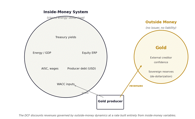
Figure 1. Conceptual schematic of the architectural mismatch. The gold producer operates across the boundary between the inside-money system (which governs costs and the WACC inputs) and the outside-money sphere (which governs revenues). The standard DCF model treats both sides as living within the same monetary reference frame.

The price of outside money is not determined by the productivity of the closed energy-dollar loop[2].

It is determined by the confidence that external creditors place in the loop’s capacity to honor its obligations in units of comparable purchasing power. When that confidence is high, outside money trades quietly. Its opportunity cost, the yield it does not pay, is high. Rational actors prefer inside money that compounds within the loop. When confidence erodes, when the external obligations of the closed loop grow faster than its real productive capacity, or when the weaponization of dollar reserves reveals that those reserves are conditional rather than unconditional, outside money rises. Not as a reflection of economic growth. Not as a reflection of inflation in the CPI sense. As a measure of the widening distance between what the loop promises and what it can deliver.

The historical record documents this mechanism with consistency. From 1971 to 1980, following the collapse of Bretton Woods and persistent external deficits financed by foreign creditors, gold rose from $35 to $850 per ounce (more than 2,300 percent in nominal terms) while the consumer price index roughly doubled. From 2000 to 2011, amid two wars, a financial crisis, and an unprecedented monetary expansion, gold climbed from $255 to $1,900. From 2018 to 2026, as dollar reserves were frozen to enforce sanctions and sovereign creditors absorbed the lesson that their holdings were subject to political conditions, gold moved from US$1,200 to above US$4,500, reaching a documented LBMA AM auction price of US$5,093.55 on January 26, 2026, and remaining above US$5,000 for more than seventy percent of auction sessions through March 17 of that year. In each episode, the all-in sustaining costs of gold production rose with general inflation in the energy economy: wages, diesel, electricity, and reagents all tracked the dollar price level. The revenue responded to an entirely different signal. The margin expanded, dramatically, because the two sides of the income statement were governed by different mechanisms.

This is the structural mismatch that the discounted cash flow model cannot see.

The free cash flow of a gold mining company is the difference between revenues driven by outside-money dynamics and costs driven entirely by inside-money dynamics. These two components respond to different shocks, different regimes, and different time horizons. In stable monetary environments, when external confidence in the loop is intact, they move roughly in parallel and the DCF produces defensible results. In the scenarios that matter most for long-term valuation (sustained monetary expansion, fiscal dominance, or accelerating de-dollarization), they diverge sharply and the DCF produces systematically wrong answers.

The discount rate applied to this difference is constructed entirely from inside-money variables: Treasury yields, dollar equity risk premia, betas measured against dollar-denominated indices. It correctly captures the cost of capital within the closed loop. It is constitutionally incapable of capturing the dynamics of the outside money that governs the revenue line.

The consequence is not random error. It is directional, persistent, and largest precisely in the scenarios where the asset’s value is highest. A model that undervalues most severely when the underlying is most valuable is not merely imprecise. It is systematically misleading.

The magnitude of this distortion, and what can be done about it, is the subject of the sections that follow.

Section IV — The Mechanism and Magnitude of the Error

An argument without a number is a conviction. This paper claims to be something more.

The structural mismatch identified in the preceding sections, revenues governed by outside-money dynamics, costs anchored in the inside-money system, both discounted at a rate constructed entirely within that system, produces a quantifiable distortion. Quantifiable not merely in theory but in the data that any analyst can access, in the transactions that professional acquirers have executed, and in the market prices that have persisted, stubbornly, below levels that any honest reading of the fundamentals would justify.

The distortion operates through two channels, distinct in their mechanism though related in their cause. Both push valuation in the same direction. Both are invisible to the standard model. Their combined effect is not a rounding error. It is a systematic repricing of an entire asset class. A formal decomposition of the error in standard asset pricing notation is provided in Appendix A; the present section develops the argument empirically.

The first channel: the numerator.

The free cash flow of a gold mining company is the product of a volume, ounces produced, and a margin, the spread between the gold price and the all-in sustaining cost. Both are projected forward over the life of the mine, typically fifteen to twenty-five years, and discounted at the WACC.

The gold price assumption in a standard DCF is derived from one of three sources: the current spot price, a consensus sell-side forecast, or a long-run equilibrium estimate. All three share the same flaw. They are calibrated on a framework, typically, the relationship between gold and real interest rates, that ceased to explain observed gold price movements after the Federal Reserve began raising rates in 2022.

The collapse is now documented across multiple independent institutional sources. RBC Wealth Management (June 2025) reports the R-squared between the gold price and the ten-year TIPS yield falling from 84 percent over 2005–2021 to 3 percent in 2022–2023 and 7 percent in 2024 through mid-2025. Apollo’s chief economist Torsten Slok (February 2026) has documented the same breakdown using independent data, characterizing it as a phenomenon that has frustrated the quant community since the Fed began its hiking cycle in 2022. S&P Global Market Intelligence (March 2025) has tracked the same phenomenon under the heading “Treasury Yields and Gold Prices: Breaking Expectations,” noting the persistence of elevated gold prices through a multi-year period of monetary tightening that, under the prior framework, should have produced sustained price weakness.

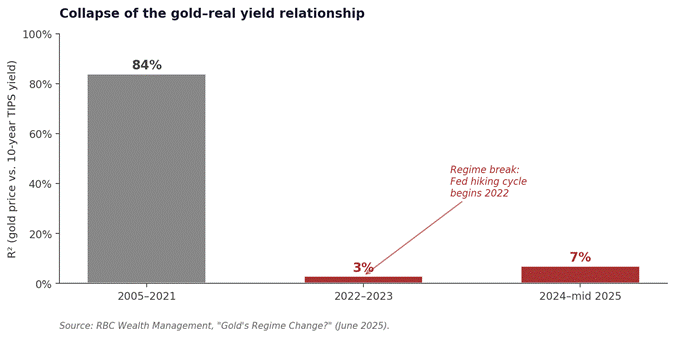
Figure 2. Collapse of the gold-real yield relationship. The R-squared between gold and the 10-year TIPS yield falls from 84% over 2005–2021 to 3–7% post-2022. Source: RBC Wealth Management.

Most directly, the World Gold Council (June 2025) has published an institutional analysis under the heading “Are Fiscal Concerns Driving Gold?” The analysis regresses gold returns against the U.S. Treasury swap-spread, a market-based proxy for fiscal stress that captures investors’ unwillingness to absorb sovereign debt issuance at prevailing prices, and finds the swap-spread statistically significant in explaining gold price movements over the period 2022 through 2025. The mechanism the WGC documents is precisely the mechanism this paper identifies: gold responds to the degradation of external confidence in the sovereign’s capacity to service its obligations, not to real interest rates as such.

Four independent institutional analyses, using different data, different periods, and different methodologies, arrive at the same conclusion. The dominant analytical framework for gold price forecasting no longer explains observed prices. The forecasts it continues to generate are artifacts of a relationship that the data themselves have ceased to support. An academic literature is emerging that examines the same phenomenon through regime-switching models, wavelet methods, and time-varying parameters; this paper relies on institutional documentation as the most directly verifiable basis for the empirical claim.

What replaced the prior framework is the mechanism described in Section III: sovereign accumulation, de-dollarization pressure, and the progressive withdrawal of external creditor confidence from dollar-denominated assets. The World Gold Council reports central bank gold purchases of 1,082 tonnes in 2022, 1,037 tonnes in 2023, and approximately 1,045 tonnes in 2024, a cumulative three-year total of roughly 3,164 tonnes, more than double the 2010–2021 average annual pace of 473 tonnes. Full-year 2025 purchases moderated to 863 tonnes, partly reflecting price-sensitive restraint by some buyers in the face of record nominal levels, but remaining well above the long-term historical norm. Independent estimates of unreported PBoC accumulation suggest that disclosed Chinese reserves significantly understate true holdings[3]. The aggregate signal is unambiguous: official-sector buying is structural, sustained, and broad-based across emerging market central banks. It does not respond to real interest rates. It responds to the architecture of the international monetary system.

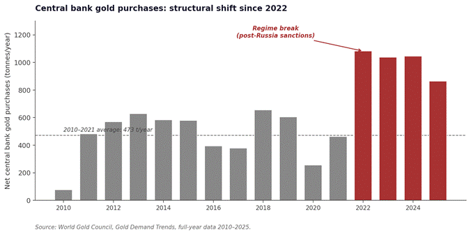
Figure 3. Central bank gold purchases 2010–2025 (tonnes/year). Net purchases since 2022 average more than double the 2010–2021 baseline of 473 tonnes/year. Source: World Gold Council, Gold Demand Trends.

A DCF model built with a gold price assumption derived from a broken analytical framework will systematically underestimate revenues. Over a twenty-year projection, a gold price that compounds at the rate of monetary expansion, conservatively estimated at four to five percent annually given global M2 trajectories, rather than reverting to a consensus equilibrium produces revenues that are dramatically higher in nominal terms. The difference, discounted back at even a standard WACC, is not marginal. It is transformative.

Three case studies across the producer spectrum.

To illustrate the magnitude of the distortion and its variation across the producer spectrum, the paper examines three cases at different points of the balance-sheet and operational continuum: a junior pre-production developer (GoldMining Inc.), a mid-tier operating producer (Equinox Gold post-Calibre acquisition), and the senior majors (Newmont, Barrick). The cases were selected to test the predicted relationship between exposure to dollar-denominated debt and the magnitude of architectural mispricing.

The junior case anchors the lower bound. On April 28, 2026, GoldMining Inc. published an updated Preliminary Economic Assessment for its La Mina project in Colombia, filed on SEDAR+ and independently prepared. The PEA presents two scenarios. The base case, using US$3,500 per ounce gold, US$4.70 per pound copper, US$40 per ounce silver, produces an after-tax NPV of US$1.0 billion at a five percent discount rate and an IRR of 32.2 percent, with all-in sustaining costs estimated at US$1,045 per ounce. The spot-price scenario, using US$4,775 per ounce gold, US$5.75 per pound copper, US$77 per ounce silver, produces an after-tax NPV of US$1.8 billion and an IRR of 49.1 percent. GoldMining’s fully diluted market capitalization on the date of publication was approximately US$252 million, based on Bloomberg-tabulated share count and closing price. La Mina represents roughly nine percent of the company’s measured and indicated gold-equivalent resources. A sum-of-the-parts analysis applying even conservative development-stage discount factors to the full portfolio produces a net asset value substantially above the market capitalization. The price-to-NAV ratio implied is approximately 0.4 to 0.5, a discount of roughly half from the conservative NAV of the development assets, before considering the optionality of the broader resource base. GoldMining carries no material long-term debt; the architectural mispricing is undiluted by balance-sheet risk.

The mid-tier case, Equinox Gold (post-Calibre acquisition completed June 2025), sits in the middle of the spectrum. Standalone 2024 production was approximately 590–675 thousand ounces; 2025 guidance for the combined entity is 785–915 thousand ounces. AISC trends are instructive: the YTD Q3 2025 figure of US$1,994 per ounce reflects the Greenstone ramp-up rather than a steady-state cost structure. Net debt at end of Q1 2025 (pre-Calibre merger) stood at approximately US$1.2 billion. Post-merger Q3 2025 net debt was US$1.28 billion, and the company subsequently reduced debt by more than US$1.1 billion since Q2 2025, ending January 2026 with cash of US$440 million against debt of US$515 million. TD Securities (July 2025) estimates Equinox trading at approximately a 30 percent discount to intermediate peers on spot P/NAV. The narrowing of dollar-debt exposure through 2025–2026 is itself consistent with the architectural prediction: as the dollar-debt counterweight shrinks, the residual mispricing should widen, not contract.

The senior majors anchor the upper bound. Newmont (NYSE: NEM) reported full-year 2024 attributable production of 6.8 million gold ounces at realized AISC of approximately US$1,500 per ounce on a consolidated basis (the quarterly trajectory ran $1,439 / $1,562 / $1,611 / $1,463 from Q1 to Q4), with long-term debt of US$7.94 billion and reported net-debt-to-adjusted-EBITDA of 0.6x. Barrick (NYSE: B) reported 2024 attributable production of 3.91 million ounces at realized AISC of US$1,484 per ounce, total debt of US$4.72 billion, and adjusted EBITDA of US$5.19 billion. Both producers fund themselves predominantly in U.S. dollar-denominated bond markets. The 3L Capital Gold M&A Study (January 2026), examining 92 transactions of greater than US$150 million between 2020 and 2025, reports that Multi-Asset Producer transactions clear at average premiums of approximately 10 percent, indicating that public-market valuations of the largest producers approach the prices strategic acquirers are prepared to pay, with the residual gap broadly explainable by transaction-specific synergies. The architectural mispricing is at its smallest among the seniors precisely because their dollar-debt balance sheets bring inside-money exposure to the right side of the equation, partially offsetting the outside-money revenue exposure.

Table 1. Three case studies across the gold producer spectrum (May 2026).

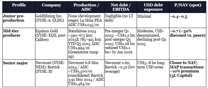
Sources: GoldMining Inc. PEA (28 April 2026, SEDAR+); Equinox Gold Corp. 6-K filings, TD Securities research note (16 July 2025); Newmont Corporation Form 10-K FY2024; Barrick Mining Corporation 2024 Annual Report; 3L Capital, “Gold M&A Note” (12 January 2026). Author calculations.

The pattern is consistent with the architectural thesis. The producer most purely exposed to outside-money revenue dynamics with no offsetting inside-money debt, the junior pre-production developer, trades at the largest discount to NAV. The producer with substantial dollar debt providing balance-sheet exposure to the inside-money side trades at a moderate discount. The senior majors, whose multi-billion dollar debt loads carry the inside-money risk in size, trade closest to NAV. The empirical signature is consistent with the theoretical prediction, though the relationship between balance-sheet dollar-debt exposure and the magnitude of architectural mispricing is inferred from the gradient across three cases rather than estimated econometrically. As balance-sheet exposure to dollar debt rises, the architectural mispricing diminishes. The magnitude of the residual mispricing across the spectrum, of order 50 percent for unleveraged juniors, ~30 percent for moderately leveraged mid-tiers, and approaching zero for highly leveraged seniors, is the empirical signature the paper identifies. Note that the three reference points draw on different observation methods (author estimate of P/NAV from PEA inputs, sell-side P/NAV discount vs. peers, M&A transaction premium vs. trading price); the convergence of the gradient is the central observation, not the perfect commensurability of the three metrics. A second qualification matters here: the gradient does not control for jurisdictional quality. The junior reference point (GoldMining, Colombia) operates in a higher-risk jurisdiction than the senior reference points (Newmont and Barrick, with substantial Nevada and Quebec exposure). A portion of the junior discount certainly reflects country risk and execution risk rather than architectural mispricing alone. The persistent P/NAV discount in the most stable jurisdictions, observed across mid-tier and senior producers operating in Nevada, Quebec, and Western Australia, is what the architectural argument cannot reduce to country risk and is therefore the residual the thesis seeks to explain. A controlled empirical test would require a sectoral regression with jurisdictional controls, which is among the open questions identified in Appendix A.4.

The second channel: the denominator.

The first channel is well-known to practitioners, even if its mechanism is poorly understood. The second is not. It operates at a deeper level than the calibration of any individual input. It concerns the structure of the pricing model itself.

The weighted average cost of capital, in its standard form, is built on a single-factor view of risk. The cost of equity is derived from the Capital Asset Pricing Model: a risk-free rate, plus a beta-weighted equity risk premium, where the beta measures the covariance of the asset’s return with the return on a market portfolio. This is the canonical formulation that every analyst learns and every institutional valuation methodology embeds. It rests on the assumption that the relevant systematic risk for any asset can be reduced to its exposure to a single factor, the market.

For most assets, this reduction is innocuous. The market factor captures, with reasonable adequacy, the dominant source of priced risk: the broad covariance of asset returns with the productive economy and the financial system that intermediates it. Industrial companies, consumer goods companies, software companies, all are exposed to this factor in roughly proportional ways. Their cost of equity, derived from a market-only beta, is approximately right.

For gold mining companies, this reduction fails, not because the market beta is wrongly measured, but because it is structurally insufficient. The relevant risk for a gold mining revenue stream is not the broad market risk that the CAPM is built to price. It is the risk of monetary regime stress: the risk that the closed energy-dollar loop’s external obligations exceed its capacity to honor them, that confidence in the dominant unit of account erodes, that the system that the WACC takes for granted as a stable reference frame is itself the variable in motion. This risk is real, priced, and orthogonal to broad market risk. It is exactly the risk to which gold revenues are negatively exposed by the mechanism described in Section III.

In a multi-factor pricing framework (Arbitrage Pricing Theory of Ross 1976, the Fama-French extensions, or any formulation that recognizes more than one priced source of systematic risk), this exposure would be captured explicitly[4]. The cost of capital for an asset negatively exposed to monetary regime risk would be lower than its single-factor counterpart, by an amount equal to the product of its monetary-factor beta and the price of monetary regime risk. The asset’s protective property (its negative covariance with the dominant macro stress of the era) would translate, mechanically, into a reduced required return.

The orthogonality of the monetary regime factor to the standard market factor warrants a brief note. The market factor that the CAPM beta measures captures covariance with broad equity returns, a measure of exposure to growth, earnings, and credit conditions within the productive economy. The monetary regime factor, by contrast, captures exposure to the level and stability of the unit of account in which the productive economy is denominated. These are by construction non-collinear: the first is a factor of growth within the system, the second is a factor of the system itself. The empirical record supports this distinction. Over multi-decade periods, gold returns exhibit low-to-negative correlation with broad equity returns precisely during episodes of monetary regime stress, the very episodes that drive the negative β_monetary loading. A market beta that captures average covariance with equity returns cannot, by construction, replicate this regime-conditional behavior.

The standard WACC contains no such adjustment. It is not that the existing market beta is wrong. It is that the model, by construction, recognizes only one factor, and the factor that matters most for this asset class is not represented at all. The error is not one of calibration. It is one of model specification.

The consequence is the same as what an erroneous beta sign would produce: a discount rate that is structurally too high for revenues whose true risk profile improves the portfolio of any investor exposed to monetary regime stress, which, in the current era, is every dollar-based investor. But the diagnosis is more precise, and more difficult to dismiss. A defender of the standard model cannot argue that “the beta already captures it”, because the beta in question, by construction, captures only a different factor. The omission is not a matter of degree. It is a matter of structure.

What the WACC measures, it measures correctly. What it does not measure, it cannot measure. And what it does not measure is precisely the dominant risk factor governing the revenue stream of the asset class under analysis.

The combined effect.

Two errors in the same valuation, both pushing in the same direction, both invisible to the standard model. The numerator is systematically underestimated because the gold price assumption is calibrated on an analytical framework whose explanatory power has collapsed. The denominator is systematically too high because the model is structurally blind to the factor that governs the revenue line.

These two errors share a common origin: a single-factor view of monetary reality in a world where the factor that matters most is no longer reducible to the variables the model contains. They are two manifestations of the same blindness, expressed at different points in the valuation arithmetic. Their combined effect is not the simple arithmetic sum of the two corrections taken in isolation: the formal decomposition presented in Appendix A makes the interaction explicit. What this paper claims is that both errors exist, that both push valuation in the same direction, and that the combined effect is large enough to plausibly account for the persistent valuation gap that the data document. The two channels are not symmetrically established. The numerator channel is documented by four independent institutional sources (RBC, Apollo, S&P Global, World Gold Council) using different methodologies on different periods, all converging on the same regime break post-2022. The denominator channel is structurally identified by the architecture of single-factor pricing but not empirically quantified in this paper: the omission of a monetary regime factor is demonstrable from the form of the standard model, but the magnitude of its effect on individual producer valuations awaits the calibrated estimation flagged in Appendix A.4. The thesis on the existence of both errors stands; the precise apportionment of the empirical valuation gap between the two channels remains an open empirical question.

What is not in question is the direction of the error or the regime in which it is largest. The combined distortion compounds precisely in the scenarios where the investment thesis is most compelling: sustained monetary expansion, fiscal dominance, accelerating de-dollarization, negative real rates. The model is most wrong when the opportunity is greatest. This is the empirical signature that the data confirm.

The mechanism of the convexity is itself worth noting. As the monetary regime deteriorates, two effects compound. First, gold prices accelerate, magnifying the gap between the broken framework’s projection and the realized price (numerator effect). Second, the operational leverage of mining producers, fixed costs against rising revenues, amplifies the impact of any percentage error in the price assumption on cash flows. The mispricing is convex in regime stress: it grows faster than linearly as monetary conditions deteriorate, which is precisely why the gap between sell-side DCF outputs and in-situ M&A pricing has widened, rather than closed, throughout the post-2022 regime.

It explains the persistent P/NAV discount across the gold mining sector. It explains why strategic acquirers have paid accelerating prices per in-situ ounce in every year since 2020 while public market valuations have lagged. The acquirers are not using a different valuation framework. They are using the same DCF architecture with different inputs and different institutional constraints, a point developed in the next section. The persistent gap between their prices and the prices implied by sell-side models is not the alpha of the position. It is the empirical measure of the error.

Section V — The Persistence of the Error and the Path to Correction

The error is not new. It has existed in every standard DCF applied to gold producers since the 1990s. It has survived multiple bull markets, record central bank buying, and the sharpest sustained repricing of gold in modern history. The question is why it persists.

The answer is institutional. Sell-side models rely on standardized price decks, firm-wide WACC methodologies, compliance templates, and consensus benchmarks. Deviating significantly from consensus gold prices or proposing a lower regime-adjusted discount rate carries professional and reputational costs. The system is optimized for consistency across sectors, not for capturing monetary regime shifts. The model was built for a stable dollar unit of account. The world changed. The institutions using the model have not.

Four objections will be raised by any serious reader of the preceding argument. They deserve direct answers.

The first: the analyst can correct for this by adjusting the gold price assumption upward. This objection is the most common and the least compelling. Ad-hoc price adjustments are discretionary, non-systematic, and institutionally constrained. More importantly, they address only the first channel of distortion. They leave the second channel, the model specification error, entirely untouched. An analyst who raises the gold price to $5,000 while maintaining a single-factor WACC of eight percent has corrected the symptom without addressing the structural blindness. When the monetary environment shifts further and the next analyst inherits the model, the gold price assumption will revert toward consensus. The correction is not durable because it is not grounded in a mechanism.

The second: the real options methodology already addresses this problem. Brennan and Schwartz formalized real options for mining assets in 1985. Dixit and Pindyck extended the framework in 1994. But real options address a different problem. They capture the value of managerial flexibility in the face of price uncertainty, the right to delay, expand, or abandon production. They do not address the distribution from which future gold prices are drawn. If that distribution is miscalibrated because the underlying price process has shifted regime, the real options model inherits the same miscalibration. The critique is orthogonal to the options literature, not superseded by it.

The third: a low market beta already partially compensates for the outside-money dynamics. Partially, and inadequately. The observed beta captures short-term covariance with equity markets and liquidity-driven sell-offs. The relevant exposure, the negative loading on monetary regime risk over a fifteen-to-twenty-year horizon, is not a function of equity covariance. It is a separate factor, orthogonal to the market factor that the beta measures. A low market beta cannot substitute for the absence of a monetary-factor term in the pricing equation. It compensates, at most, for a small fraction of the structural error described in Section IV.

The fourth: if the model were systematically wrong, arbitrageurs would close the gap. Persistent P/NAV discounts at typical sector levels ignore real frictions: sector illiquidity, restrictive institutional mandates, long required holding periods, and career risk for contrarian positions. Correction is occurring, rising M&A multiples, improving equity performance since 2022, but at the slow pace of institutional capital.

On Erb and Harvey: a horizon distinction.

A fifth objection deserves separate treatment because it comes from a serious academic source. Erb and Harvey, in “The Golden Dilemma” (Financial Analysts Journal, 2013), document that gold is a poor inflation hedge over short and intermediate horizons (one to ten years), that the real price of gold is mean-reverting on a long-run basis, and that historical purchases at high real prices have produced poor subsequent real returns. Their statistical evidence is robust within its frame and any working paper on gold valuation that ignores it earns the criticism it will receive.

The thesis advanced here does not contradict their findings. It operates on a different mechanism and a different horizon. Erb and Harvey test gold against CPI, a measure of consumer prices within the closed energy-dollar loop. The mechanism this paper describes governs gold against the confidence external creditors place in the loop’s sustainability, a different variable that is correlated with CPI only in regimes where fiscal pressure is being transmitted through consumer prices, which has not been the dominant regime over most of the period Erb and Harvey examine. The mean reversion they document is reversion to a real price calibrated on the very framework whose explanatory power Section IV documents has collapsed since 2022. If the framework that defines “real” ceases to capture the dominant driver of the variable being deflated, mean reversion within that framework is consistent with persistent dispersion outside it.

More fundamentally, the present paper makes no claim about whether gold is a good investment for any particular investor at any particular price. It claims that the standard DCF, applied to gold mining companies, contains a structural mismatch between the monetary regime governing revenues and the monetary regime embedded in the discount rate. This mismatch produces undervaluation of producers relative to in-situ acquisition prices regardless of whether one believes gold itself is fairly valued, expensively valued, or cheaply valued at any moment. The Erb-Harvey caution applies to the investor deciding whether to hold gold; the architectural argument applies to the analyst deciding whether the DCF correctly prices gold producers. These are not the same question. A reader who finds Erb and Harvey persuasive on the first question can still find the architectural argument persuasive on the second, they address different objects.

Where Erb and Harvey would directly invalidate this paper is in a regime where the gold-CPI relationship reasserts itself, real interest rates return to substantially positive territory, and the post-2022 break in the gold-real-yield correlation reverses. Section VI specifies precisely this condition. If it materializes, the multi-factor framework collapses to its single-factor limit and the standard DCF recovers its validity. Until it does, the architectural argument stands.

Operational and balance-sheet risks: the dollar-debt counterweight, quantified.

Before turning to the empirical correction the market has produced, one further qualification is necessary. Gold is outside money. A gold mining company is not. Producers are industrial entities embedded in the inside-money system at every level: their workforce, their energy supply, their permitting, their tax exposure, and, critically, their balance sheet.

The dollar debt of major gold producers is a particularly serious counterweight to the outside-money exposure of their revenues. The major producers (Newmont, Barrick, Agnico Eagle, and the mid-cap operators) fund themselves predominantly in dollar-denominated bond and credit markets. The magnitude of this exposure is no longer abstract. As of full-year 2024, Newmont reported long-term debt of approximately US$7.94 billion against attributable EBITDA implying a reported net-debt-to-adjusted-EBITDA ratio of 0.6x. Barrick reported total debt of US$4.72 billion against adjusted EBITDA of US$5.19 billion. The mid-tier Equinox Gold reported pre-merger net debt of approximately US$1.2 billion at end of Q1 2025 against pro-forma annualized revenue approaching US$4 billion at current spot prices. These are not the balance sheets of small operators: they are multi-billion-dollar dollar-denominated obligations that must be serviced regardless of the metal’s monetary trajectory.

The Equinox case is also instructive on the dynamic nature of the counterweight. Through 2025 and into 2026, the company reduced debt by more than US$1.1 billion and ended January 2026 with cash of US$440 million against debt of US$515 million. As the dollar-debt offset shrinks, the architectural mispricing the firm carries should, on the thesis advanced here, expand rather than compress, a testable implication that subsequent quarters of P/NAV evolution will validate or contradict.

In monetary regimes where the dollar weakens against gold but strengthens against other currencies, the real burden of these liabilities can expand at precisely the moment when production economics deteriorate in local-currency terms. This is the structural asymmetry of a producer compared to physical gold: the metal has no liability side of its balance sheet; the producer carries one, denominated in the very currency whose erosion gives the metal its value. The senior major thus operates partially as a hedge of its own monetary exposure: the dollar liabilities offset, in part, the dollar revenues that would otherwise be undervalued by the standard discount rate.

This is a real counterweight, not a refutation. It does not eliminate the architectural error in the DCF, the producer’s revenues remain governed by outside-money dynamics, and the standard discount rate remains structurally blind to them. But it limits the magnitude of the mispricing the architectural argument can claim, and it explains the empirical pattern documented in the case studies (Table 1): the architectural mispricing is largest among unleveraged juniors and progressively dampens as dollar-debt exposure rises through the producer spectrum. The market is partially pricing the dollar-debt risk that the in-situ method ignores.

The empirical correction: in-situ valuation as an unconstrained DCF aggregate.

The practitioners who write acquisition checks have already begun to correct the error empirically, without naming it. Their method deserves precise description.

Strategic acquirers do not abandon the DCF. Corporate development teams at major producers run discounted cash flow models on every target they evaluate. The architecture is the same as the sell-side architecture. What differs is everything else: their inputs are not bound by firm-wide commodity price decks, their discount rates are not imposed by valuation methodology teams optimizing for cross-sector comparability, their time horizon is the operational life of the asset rather than the duration of an analyst’s coverage, and their reference points are recent transactions in the same market, not consensus forecasts.

The in-situ price per ounce that emerges from the M&A market is the empirical aggregate of these unconstrained DCFs. It is not a separate valuation method standing in opposition to the DCF. It is the DCF, applied with inputs that the institutional sell-side process is structurally incapable of generating. The persistence of the gap between in-situ prices and sell-side valuations is therefore not evidence that the DCF is wrong as a method. It is evidence that the inputs the DCF receives in standardized institutional settings are wrong.

The in-situ approach has limitations that should be stated plainly. It depends on comparable transactions, and the universe of comparables is small at any moment. It applies a price per ounce that does not, by itself, distinguish between a project requiring $800 of capex per ounce of development and one requiring $5,000. It captures a temporal aggregate that lags any sudden regime shift. The dispersion of in-situ prices at any single moment (from below $80 per ounce for early-stage exploration to above $170 per ounce for permitted, near-production projects) is wide enough that “the in-situ price” is a distribution, not a single number.

A more fundamental limitation deserves explicit acknowledgement. The argument that the in-situ aggregate represents the architecturally-correct DCF is not without circularity. M&A premia incorporate factors beyond price discovery: operational synergies that the standalone target cannot realize, portfolio considerations of the acquirer, the avoided cost of multi-year development for already-permitted assets, and strategic positioning within a sector. A reader could reasonably argue that the gap between sell-side valuations and M&A prices reflects these factors rather than monetary regime mispricing per se. The architectural argument cannot fully discriminate between the two interpretations from the empirical record alone. What can be said is that the gap exists, that it has widened in the post-2022 regime where the architectural mismatch is most acute, and that its directional consistency across the producer spectrum is consistent with the thesis advanced here. The discrimination between architectural mispricing and acquisition-specific premia is precisely the kind of question that calibrated estimation of the corrected pricing model (Appendix A.4) would resolve.

These limitations argue for using in-situ as triangulation rather than replacement. When a sell-side DCF and the in-situ aggregate produce values within a defensible range of each other, the institutional consensus is functioning. When they diverge by a factor of two or three, as they routinely do in the current environment, the divergence is a signal worth investigating, and the investigation returns to the inputs.

The trajectory of the data is unmistakable. The World Gold Council and S&P Global have tracked in-situ transaction prices systematically. The 2020 median was approximately $80 per ounce. By 2024 the Australian average had reached $122. The unsolicited Fujairah-Asante offer of 2023 implied $177 per ounce[5]. The Equinox-Gold acquisition of Calibre Mining was announced in February 2025 at approximately $1.8 billion and completed in June 2025 at an implied transaction value of approximately $2.56 billion, reflecting the appreciation of Equinox shares between announcement and closing. By early 2026, 3L Capital reports developer reserve transactions averaging $230 per ounce, with single-asset producer deals clearing at premiums of approximately 35 percent.

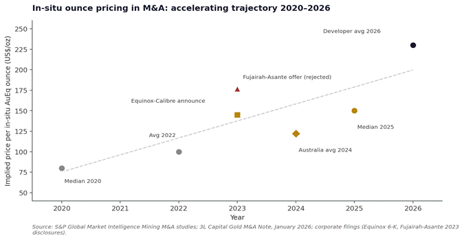
Figure 4. In-situ ounce pricing in M&A 2020–2026. The trajectory documents the accelerating willingness of strategic acquirers to pay for ounces in the ground, while public-market valuations of comparable assets have lagged. Sources: S&P Global Mining M&A studies; 3L Capital Gold M&A Note (January 2026); corporate filings.

Strategic acquirers, including those whose offers have not been accepted, are signaling accelerating willingness to pay for ounces in the ground, in a period during which the public valuations of comparable assets have lagged. The persistent gap is the empirical signature of the institutional friction this section has described. The point is not that acquirers have found a better answer than analysts. It is that they are using a process less encumbered by the institutional pressures that produce convergence on broken inputs. When their valuations and sell-side models diverge persistently and directionally, the divergence is itself the data. Treating it as such is what this paper proposes.

The direction of the formal correction is clear, even if its precise mathematical specification lies beyond the scope of this paper. The discount rate applied to gold mining cash flows should be derived from a multi-factor pricing framework that recognizes monetary regime risk, in the precise sense of fiscal dominance[6], as a priced factor distinct from market risk. The cost component of the cash flow can retain its conventional WACC treatment. The revenue component requires a discount rate that reflects its true risk profile: negatively correlated with monetary regime stress, positively correlated with the degradation of external confidence in the closed loop. Collapsing both into a single uniform rate derived from a single-factor model will continue to produce the same answer it has always produced.

Precise. Internally consistent. And wrong.

Section VI — Testable Predictions and Conditions of Falsification

An analysis that cannot be wrong is not analysis. It is advocacy.

The preceding sections advance a structural argument: that the discounted cash flow model, as applied to gold mining companies, contains an architectural error, a misspecified price assumption in the numerator and a misspecified pricing model in the denominator, that produces systematic undervaluation. This argument has implications that are testable. It makes predictions about what should happen if the mechanism is real. And it specifies, with equal precision, the conditions under which it would be wrong.

Both matter. A thesis that lists only its confirmations and ignores its invalidations is a brief, not a paper. What follows is a statement of both.

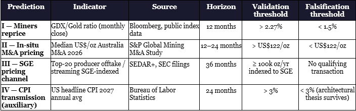
Prediction I — The miners reprice relative to the metal.

The GDX-to-gold spread, the ratio of the gold miners index to the gold price, currently stands near its historical lows. Momentum Structural Analysis has identified 2.27 percent as the breakout level on a monthly close basis: the threshold above which miners have historically begun to dramatically reprice relative to gold. If the architectural error identified in this paper is real and is being progressively recognized by the market, the spread should break above this level within twelve months of this writing.

Invalidation condition:

If the GDX-to-gold spread fails to break above 2.27 percent and instead compresses below 1.5 percent on a monthly close basis, the thesis is premature.

Prediction II — Strategic acquirers continue to price in-situ ounces at record levels.

If the in-situ aggregate captures inputs that sell-side processes systematically fail to generate, the prices paid per in-situ ounce in M&A transactions should continue to rise throughout 2026 and 2027. S&P Global’s annual mining M&A studies provide the benchmark: the 2024 average for Australian transactions was approximately $122 per ounce. The thesis predicts that the 2026 study will show a number above this level.

Invalidation condition:

If the average price per in-situ ounce in S&P Global’s 2026 M&A study falls below the 2024 level, the thesis is weakened.

Prediction III — The physical pricing channel displaces the paper channel.

The argument that gold is priced as outside money implies that the Shanghai Gold Exchange, which settles in yuan and reflects physical supply and demand, should progressively gain relevance. At least one top-twenty global gold producer (by annual production) should announce, within thirty-six months of this writing, an offtake or streaming agreement of at least 100,000 ounces per year explicitly indexed to the SGE price rather than the COMEX price.

Invalidation condition:

If no such transaction is announced within thirty-six months meeting both the producer-size and contract-size thresholds, this specific element of the thesis is not confirmed.

Prediction IV — The monetary transmission mechanism confirms itself.

The argument that gold responds to monetary expansion rather than to CPI inflation implies that the expansion of global M2 since 2019 should eventually transmit to the general price level in a manner that exceeds consensus. If the monetary mechanism is real, the 2027 headline inflation print in the United States should exceed three percent, conditional on M2 remaining on its current trajectory and the absence of an offsetting collapse in monetary velocity. This prediction is auxiliary and not required for the core architectural thesis. Its weakness reflects the genuine difficulty of forecasting M2-CPI transmission, which is mediated by velocity, output gap, and fiscal posture in ways that are not fully predictable.

Invalidation condition:

If 2027 headline CPI averages below three percent despite continued M2 expansion, the transmission mechanism is weaker than the thesis assumes. The architectural argument survives this invalidation, but the specific monetary driver claim is weakened.

Table 2. Summary of falsifiable predictions, with indicators, sources, horizons, and validation/falsification thresholds.

The condition under which the central thesis is invalidated.

The four predictions above test whether the market is progressively correcting the mispricing identified in this paper. They do not test whether the architectural argument itself is wrong. That test requires a different condition.

The central thesis rests on the claim that gold revenues and gold mining costs respond to different mechanisms, and that the standard discount rate is constructed from a single-factor model that omits the priced factor governing the revenue mechanism. This claim would be empirically refuted if the relationship between gold prices and real interest rates, the TIPS-gold R-squared, were to be restored to its pre-2022 level of above sixty percent on a sustained basis over five years.

Such a restoration would require a return to substantially positive real rates, somewhere in the range of three to four percent sustained over a business cycle, comparable to the Volcker-Greenspan era of 1982 to 2000. In that regime, the gold price is once again primarily determined by the opportunity cost of holding a non-yielding asset within the closed loop, rather than by the confidence of external creditors in the loop’s sustainability. The single-factor WACC, calibrated on inside-money variables, would again correctly capture the dominant driver of gold revenues, and the multi-factor extension proposed in this paper would reduce to its single-factor limit.

This scenario has a real-world price: sustaining real rates of three to four percent in an environment where sovereign debt stands above one hundred percent of GDP in every major advanced economy would require either a dramatic fiscal contraction, a severe recession that destroys private credit, or a political decision to impose losses on creditors through restructuring. Each of these paths is observable. None is impossible. If any materializes and sustains, the thesis deserves to be revisited.

The thesis does not predict that this scenario cannot occur. It predicts that the political and institutional cost of producing it is high enough that the probability distribution of outcomes over a fifteen-to-twenty-year horizon, the exact horizon of the DCF models under critique, is weighted toward continued monetary expansion and continued outside-money dynamics. That is a probabilistic claim, not a certainty. Probabilistic claims can be wrong.

If they are, the paper will say so.

Conclusion — The Architecture of the Error

This paper has advanced a single, precise claim: the discounted cash flow model, as conventionally applied to gold mining companies, contains a structural, architectural error that cannot be fully corrected by adjusting inputs. Revenues governed by outside-money dynamics are projected from a forecasting framework whose explanatory power has collapsed, and discounted at a rate built from a single-factor model that omits the very factor governing those revenues. The numerator and the denominator do not share a common monetary reference frame. The resulting undervaluation is systematic, directional, and largest precisely when the protective characteristics of gold are most valuable.

Two clarifications close the argument.

Gold is outside money; a gold mining company is not. The architectural mismatch coexists with real operational and balance-sheet risks (dollar-denominated debt foremost among them) that are partially captured in country risk premia and credit spreads. These risks limit the magnitude of the architectural mispricing the thesis can claim. They do not eliminate it: the persistent P/NAV discount in the most stable jurisdictions (Nevada, Quebec, Western Australia) cannot be explained by jurisdictional risk alone.

The two errors identified in this paper also share a common origin, and their combined effect is not a simple arithmetic sum. The formal decomposition presented in Appendix A makes the structure of the interaction explicit. What the paper claims is that both errors exist, that both push valuation in the same direction, and that their combined empirical signature is the persistent gap between standardized DCF outputs and the in-situ prices paid by acquirers operating outside the institutional constraints of sell-side research.

The practical implication is not to buy or sell gold equities. It is to recognize the limitations of the dominant valuation tool. The DCF will remain in use for institutional, compliance, and standardization reasons. But those who rely on it should understand what it cannot see: that the revenue line of a gold producer responds to a priced risk factor that the standard cost of capital, by structural design, does not contain. They should understand that the in-situ aggregate represents the same valuation architecture run with inputs that the institutional process is incapable of generating, and that its persistent divergence from sell-side outputs is data, not noise.

Closing the gap, through differentiated discount rates derived from multi-factor frameworks, through better regime-aware inputs in the price assumptions, or through greater humility about the domain of validity of the standard tool, is the work that follows from this paper.

The thermometer still reads a number. For this class of assets, understanding why the number is systematically wrong is the beginning of getting the value right.

Appendix A — Formal Decomposition of the Error

This appendix presents a formal decomposition of the error identified in the body of the paper. The treatment is intentionally compact. It identifies the structural form of the corrected valuation, the parameters whose calibration is required for empirical implementation, and the qualitative direction of each correction. A rigorous econometric estimation of the parameters is the work of subsequent research.

A.1 — The standard DCF specification.

Under the standard single-factor framework, the value of a gold mining company at time zero is given by:

V_DCF = Σ_t [FCF_t(P_gold,t) / (1 + WACC)ˆt]

where FCF_t denotes free cash flow at time t, P_gold,t is the projected gold price, and WACC is the weighted average cost of capital derived from a single-factor (CAPM) model. Standard inputs typically take P_gold,t to be a constant (consensus deck) or to grow at the rate of expected CPI inflation; WACC is constructed as R_f + β_mkt · λ_mkt for the equity component, blended with after-tax cost of debt at corporate weights. For major gold producers in current data, this produces a WACC in the range of 7.5 to 9 percent.

A.2 — The corrected specification.

The architectural correction recognizes that revenues and costs respond to different factor structures. Define the corrected value as:

V_correct = Σ_t [Rev_t(P_gold,t) / (1 + r_revenue)ˆt] − Σ_t [Cost_t / (1 + r_cost)ˆt]

where Rev_t and Cost_t denote revenues and costs respectively, and the discount rates differ:

r_revenue = R_f + β_mkt · λ_mkt + β_monetary · λ_monetary

r_cost = WACC (standard, single-factor)

The new term β_monetary · λ_monetary captures the loading on monetary regime risk, where β_monetary is the sensitivity of gold revenues to the monetary regime factor and λ_monetary is the price of bearing that risk. For an asset whose revenues rise when monetary regime stress increases (gold), β_monetary < 0; for any reasonable specification of λ_monetary > 0, the second term reduces r_revenue below the single-factor WACC. The numerator path P_gold,t is itself revised upward, reflecting the regime-aware projection rather than the consensus deck calibrated on the broken framework. The sign assumption β_monetary < 0 is theoretically motivated by the mechanism described in Section III but is not empirically estimated in this paper; its sign is the structural prediction whose empirical confirmation would render the multi-factor specification operational.

A.3 — Decomposition of the error.

The total error E induced by the standard model relative to the corrected specification can be written as:

E = V_correct − V_DCF = E_numerator + E_denominator + E_interaction

where E_numerator captures the effect of replacing the broken price projection with a regime-aware path (ΔP_gold), E_denominator captures the effect of replacing the single-factor WACC with the multi-factor revenue discount rate (Δr), and E_interaction captures the cross-effect, which is non-zero because both adjustments operate on the same projected cash flow stream. The interaction term is generally positive in the regime under analysis: the higher revenue path is discounted at a lower rate, amplifying the present-value impact of each correction.

The qualitative result is unambiguous: under any specification with β_monetary < 0 and a regime-aware P_gold path that exceeds the consensus deck, all three components of E are positive. The combined error is therefore positive and pushes the corrected valuation above the standard DCF in the same direction. The empirical magnitude of E across the producer spectrum is documented in the case studies of Section IV.

A.4 — Calibration challenges and direction of subsequent work.

Three empirical questions remain open. First, the appropriate proxy for the monetary regime factor, candidates include the Treasury swap-spread (used by the World Gold Council in its fiscal-driver analysis), a debasement-adjusted real yield, or a constructed factor combining sovereign reserve flows and de-dollarization metrics. Second, the estimation of β_monetary for individual producers, which requires a time series long enough to span monetary regime shifts and an instrumental approach to handle the endogeneity between gold prices and the proxy variable. Third, the specification of λ_monetary, which under standard pricing theory should reflect the price of monetary regime risk in the broader investor universe, a parameter not directly observable from any single asset class. Each of these questions is tractable in principle. None is resolved in the present paper. The contribution here is structural: identifying the omission as the source of systematic error, and proposing the form of the correction. The empirical calibration is the next step.

A Note on Operational Implications

This paper has identified an architectural error in the standard DCF as applied to gold mining companies and has documented its empirical signature. The natural question for the practitioner is what to do about it in the next valuation exercise, before the calibrated multi-factor framework that Appendix A.4 calls for becomes available.

That question deserves its own treatment. A companion note in preparation will propose three operational adjustments that practitioners can apply to their existing DCF workflow without waiting for a fully calibrated replacement: a regime-aware approach to the gold price assumption that breaks with the consensus deck calibrated on the post-2022 broken framework, a heuristic adjustment to the cost of capital that approximates the omitted monetary regime factor while remaining defensible on standard methodological grounds, and a triangulation procedure with in-situ M&A comparables that converts the persistent gap documented in Section V into an actionable diagnostic. The companion note will work through a complete numerical example on a documented mid-tier producer with recent M&A activity, showing the standard DCF and the adjusted DCF in parallel.

The diagnosis presented here is the foundation. The operational adjustments are the bridge to practice while the rigorous econometric calibration awaits its own paper.

Bibliography

References follow Chicago author-date format. Online sources accessed May 2026. The empirical claims in this paper rely on institutional documentation (RBC Wealth Management, Apollo Academy, S&P Global Market Intelligence, World Gold Council) that has been individually verified. An emerging academic literature on the post-2022 gold-real yield relationship is referenced contextually but not invoked as primary evidence.

Primary Sources and Institutional Data

3L Capital. “Gold M&A Note: Where Producers, Developers, and Capital Are Headed.” 12 January 2026.

Apollo Academy. “Gold and Rates Correlation Breakdown.” The Daily Spark by Torsten Slok, Apollo Chief Economist. 9 February 2026. https://www.apolloacademy.com/gold-and-rates-correlation-breakdown/

Barrick Mining Corporation. Annual Report 2024 (Form 40-F) and Q4/Full Year 2024 Results. 12 February 2025.

Bureau of Labor Statistics. Consumer Price Index, All Urban Consumers (CPI-U). Washington, D.C.: U.S. Department of Labor. Series CUUR0000SA0. https://www.bls.gov/cpi/

De Pessemier, Jeremy. “You Asked, We Answered: Are Fiscal Concerns Driving Gold?” World Gold Council Gold Focus blog. 24 June 2025. https://www.gold.org/goldhub/gold-focus/2025/06/you-asked-we-answered-are-fiscal-concerns-driving-gold

Equinox Gold Corp. Form 6-K, Q1 2025 Results and Acquisition of Calibre Mining Corp., completed 17 June 2025. SEC filing.

Federal Reserve Bank of St. Louis. M2 Money Supply (M2SL). FRED Economic Data. https://fred.stlouisfed.org/series/M2SL

GoldMining Inc. “Updated Preliminary Economic Assessment, La Mina Gold-Copper Project, Colombia.” Press release, 28 April 2026. Filed on SEDAR+. https://www.sedar.com

International Monetary Fund. Global Debt Database, 2024. Washington, D.C.: IMF, 2024. https://www.imf.org/external/datamapper/datasets/GDD

Metals Focus. Gold Mine Cost Service. Published quarterly in conjunction with the World Gold Council. London: Metals Focus, 2024.

Momentum Structural Analysis (Oliver, Mike). Gold Stock Monitor Weekend Report. 26 April 2026. Private circulation.

Newmont Corporation. Form 10-K FY2024. United States Securities and Exchange Commission filing, February 2025. https://www.sec.gov/cgi-bin/browse-edgar?action=getcompany&CIK=0001164727

Nieuwenhuijs, Jan. “China’s Hidden Gold Reserves.” The Gold Observer / Gainesville Coins research, 2023–2025. https://www.goldobserver.com

RBC Wealth Management. “Gold’s Regime Change?” Research note, June 2025. https://www.rbcwealthmanagement.com/en-eu/insights/golds-regime-change

S&P Global Market Intelligence. “Treasury Yields and Gold Prices: Breaking Expectations.” New York: S&P Global, March 2025.

S&P Global Market Intelligence. Mining M&A Study 2024: Trends in Transaction Prices per In-Situ Ounce. New York: S&P Global, 2024.

S&P Global Market Intelligence. FactSet Deep Sector: Metals and Mining, 2025 M&A and ECM Insights. New York: S&P Global, February 2026.

TD Securities. “Equinox Gold Corp.: Equity Research Note Post-Calibre Mining Acquisition.” 16 July 2025.

U.S. Department of the Treasury. Treasury International Capital (TIC) System: Major Foreign Holders of Treasury Securities. Washington, D.C.: U.S. Treasury. https://ticdata.treasury.gov

World Gold Council. “Are Fiscal Concerns Driving Gold?” London: World Gold Council, June 2025. https://www.gold.org/goldhub/gold-focus/2025/06/you-asked-we-answered-are-fiscal-concerns-driving-gold

World Gold Council. Gold Demand Trends: Full Year 2024. London: World Gold Council, February 2025. https://www.gold.org/goldhub/research/gold-demand-trends/gold-demand-trends-full-year-2024

World Gold Council. Gold Demand Trends: Full Year 2025. London: World Gold Council, February 2026.

World Gold Council. All-In Sustaining Cost (AISC) Data, Q3 2024. London: World Gold Council, 2024.

World Gold Council. “Beyond CPI: Gold as a Strategic Inflation Hedge.” London: World Gold Council, April 2021.

Pricing and Valuation Theory

Black, Fischer, Michael C. Jensen, and Myron Scholes. 1972. “The Capital Asset Pricing Model: Some Empirical Tests.” In Studies in the Theory of Capital Markets, edited by M. C. Jensen. New York: Praeger.

Brennan, Michael J., and Eduardo S. Schwartz. 1985. “Evaluating Natural Resource Investments.” Journal of Business 58 (2): 135–157.

Chen, Nai-Fu, Richard Roll, and Stephen A. Ross. 1986. “Economic Forces and the Stock Market.” Journal of Business 59 (3): 383–403.

Copeland, Tom, Tim Koller, and Jack Murrin. 2000. Valuation: Measuring and Managing the Value of Companies. 3rd ed. New York: McKinsey & Company / John Wiley & Sons.

Damodaran, Aswath. 2009. “Valuing Commodity Companies.” Stern School of Business Working Paper. New York: NYU.

Damodaran, Aswath. 2012. Investment Valuation: Tools and Techniques for Determining the Value of Any Asset. 3rd ed. Hoboken, NJ: John Wiley & Sons.

Dixit, Avinash K., and Robert S. Pindyck. 1994. Investment under Uncertainty. Princeton: Princeton University Press.

Fama, Eugene F., and Kenneth R. French. 1993. “Common Risk Factors in the Returns on Stocks and Bonds.” Journal of Financial Economics 33 (1): 3–56.

Petkova, Ralitsa. 2006. “Do the Fama-French Factors Proxy for Innovations in Predictive Variables?” Journal of Finance 61 (2): 581–612.

Ross, Stephen A. 1976. “The Arbitrage Theory of Capital Asset Pricing.” Journal of Economic Theory 13 (3): 341–360.

Samis, Michael, and Denis Poulin. 2012. “Using Real Options to Value and Manage Mining Projects.” Mining Engineering 64 (2): 41–46.

Gold and Monetary Economics (Background)

Baur, Dirk G., and Brian M. Lucey. 2010. “Is Gold a Hedge or a Safe Haven? An Analysis of Stocks, Bonds and Gold.” Financial Review 45 (2): 217–229.

Cheema, Muhammad A., Robert Faff, and Kenneth R. Szulczyk. 2022. “The 2008 Global Financial Crisis and COVID-19 Pandemic: How Safe Are the Safe Haven Assets?” International Review of Financial Analysis 83: 102316. https://doi.org/10.1016/j.irfa.2022.102316

Eichengreen, Barry. 2011. Exorbitant Privilege: The Rise and Fall of the Dollar and the Future of the International Monetary System. Oxford: Oxford University Press.

Erb, Claude B., and Campbell R. Harvey. 2013. “The Golden Dilemma.” Financial Analysts Journal 69 (4): 10–42.

Gurley, John G., and Edward S. Shaw. 1960. Money in a Theory of Finance. Washington, D.C.: Brookings Institution.

Jastram, Roy W. 1977. The Golden Constant: The English and American Experience, 1560–1976. New York: John Wiley & Sons. Reprint with update by Jill Leyland, Cheltenham: Edward Elgar, 2009.

Lucey, Brian M., Sile Sharma, and Samuel Vigne. 2016. “Gold and Inflation(s): A Time-Varying Relationship.” Economic Modelling 58: 633–641.

Mehrling, Perry. 2011. The New Lombard Street: How the Fed Became the Dealer of Last Resort. Princeton: Princeton University Press.

Obstfeld, Maurice, and Alan M. Taylor. 2004. Global Capital Markets: Integration, Crisis, and Growth. Cambridge: Cambridge University Press.

Reinhart, Carmen M., and Kenneth S. Rogoff. 2009. This Time Is Different: Eight Centuries of Financial Folly. Princeton: Princeton University Press.

Sargent, Thomas J., and Neil Wallace. 1981. “Some Unpleasant Monetarist Arithmetic.” Federal Reserve Bank of Minneapolis Quarterly Review 5 (3): 1–17.

Synek, Richard. 2024. “Cointegration Analysis of US M2 and Gold Price Over the Last Half Century.” European Financial and Accounting Journal 19 (1): 1–19.

Practitioner and Policy Literature

Durrett, Don. 2019. How to Invest in Gold and Silver: A Complete Introduction with a Focus on Mining Stocks. Updated 2026. GoldStockData.com.

Pozsar, Zoltan. 2022. “Bretton Woods III.” Credit Suisse Economics. 7 March 2022.

Pozsar, Zoltan. 2022. “War and Interest Rates.” Credit Suisse Global Money Notes. August 2022.

---

[1]The distinction outside money / inside money was introduced by Gurley and Shaw (1960) in Money in a Theory of Finance. The present paper extends the concept to characterize gold’s monetary properties relative to the dollar-denominated financial system, and applies it to the valuation of producers operating across the boundary between the two regimes.

[2]A standard objection to the outside-money characterization observes that rising gold prices render previously sub-economic deposits commercially viable, expanding mine supply and, through standard supply-demand mechanics, placing downward pressure on the long-term price. This dynamic is real and visible in the recalculation of pit shells at current prices. Its magnitude is nevertheless constrained by three structural features specific to gold: a stock-to-flow ratio of approximately seventy years (annual mine production representing roughly 1.5% of the above-ground stock); a monetary and reserve demand whose ceiling is not physical but contingent on confidence in the alternative system; and a marginal cost of production that is itself indexed to monetary inflation. The price elasticity of mine supply over 2010–2024, a period during which the gold price approximately quadrupled, is on the order of 0.07, an order of magnitude lower than industrial commodities. The supply-demand mechanism operates, but with a lag and an amplitude insufficient to offset outside-money dynamics over the DCF horizon. Within the DCF itself, the rising-price-extends-reserves effect is a numerator amplifier, not a denominator dampener: at higher prices, the recoverable tonnage of any given deposit expands at lower cut-off grades, increasing the present value of the asset rather than reducing it.

[3]Estimates of unreported PBoC accumulation in the 4,000–5,500 tonne range have circulated among independent gold market analysts, notably Jan Nieuwenhuijs (The Gold Observer) and others tracking the gap between Chinese gold imports, domestic mine supply, and disclosed reserve changes. These estimates are not officially endorsed by the World Gold Council or by Chinese monetary authorities. The point relevant to this paper is not the precise figure but the documented gap between disclosed and inferred holdings, which is itself a feature of the regime under analysis.

[4]The standard CAPM cost of equity is E[R_i] = R_f + β_mkt · λ_mkt, where λ_mkt is the equity risk premium. A two-factor extension recognizing monetary regime risk would write E[R_i] = R_f + β_mkt · λ_mkt + β_monetary · λ_monetary. For an asset with β_monetary < 0 and λ_monetary > 0, the second term reduces the required return relative to the single-factor benchmark. The construction of an appropriate monetary regime factor and the estimation of λ_monetary are identified as open empirical questions in Appendix A.4; their rigorous econometric calibration is left to subsequent work.

[5]The Fujairah-Asante figure cited reflects the implied per-ounce valuation of an unsolicited 2023 acquisition offer that was rejected by the Asante board. It is included here not as a completed transaction but as an observable data point on the price strategic acquirers are prepared to bid in the current monetary environment. The 2024 Fujairah-Asante Gold Forward Agreement was a separate financing transaction and is not the reference point.

[6]The term is used here in the precise sense of Sargent and Wallace (1981): a regime in which the path of fiscal policy constrains the conduct of monetary policy, such that the monetary authority cannot independently determine the price level. It is distinct from broader conditions of fiscal pressure or expansionary fiscal posture.